In the previous post we learnt that models, especially transformer based models are getting bigger and bigger by the day and hosting them for inference brings about many challenges. In this post, we’ll understand various model optimization techniques and how they can help optimize models for inference.
Optimizing statistical models for inference Link to heading
As we’ve learnt from our previous post, statistical or linear models are smaller compared to Deep Learning (DL) models. Which means, hosting linear models for inference is typically a straightforward affair. During training linear models, there is a process called hyperparameter optimization, where parameters that are optimal for the learning algorithm are set. Arriving at optimal hyperparameters for a model is an empirical process.
For linear models, a model is said to perform well when a given set of hyperparameters will result in the highest prediction accuracy for the model. Although, this is not an optimization technique that would improve inference performance, it is important to pay attention to this process during training - as hyperparameter tuning during training will result in an optimal model for inference.
Note that the optimization techniques depend on the type of statistical or linear algorithm used for building the model.
Optimizing Deep Neural Networks (DNNs) Link to heading
One of the interesting insights revealed by the machine learning research community while exploring DNNs for various tasks, is that the quality of the model increases by increasing the width (layers) and depth (nodes) of a neural network.
He et al. introduced very deep residual networks and claimed …
“We obtain [compelling accuracy] via a simple but essential concept— going deeper.”
On the other hand Zagoruyko and Komodakis argues that …
“wide residual networks are far superior over their commonly used thin and very deep counterparts.”
Not surprisingly, increasing the width (number of layers) and depth in a DNN also significantly increases the number of parameters, which in turn increases the size of the models significantly.
So, what can be done to reduce DNNs model sizes so that the compute and memory requirements can also be dialed down making it optimal for inference?
Model Compression Link to heading
Model compression is when one or more of the below techniques are used to optimize a model:
- Model Pruning (removing unimportant weights)
- Knowledge Distillation (training a smaller model to mimic a larger one)
- Model Quantization (reducing numerical precision of weights, activations)
Let’s look at each of these techniques in detail.
Model Pruning Link to heading
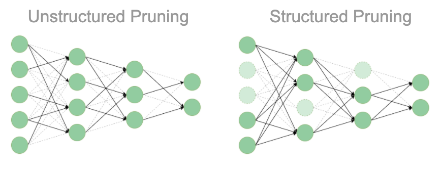
Model pruning is a technique where redundant or less important connections (weights) in a DNNs are removed or in other words pruned. Removing these less important weights from a DNN can significantly reduce the number of parameters, thereby resulting in smaller model size, thereby reducing the computational requirements to host the model for inference.
model pruning typically involves three steps:
- First, a large, DNN is trained on a given task at hand.
- The trained model is then analyzed and reduntant or less important connections (weights) that have a relatively small impact on the model’s output are pruned.
- Finally, The pruned model is then fine-tuned on the training data to regain any lost accuracy due to the pruning process.
Check out this Diving into model pruning article by weights and biases.
As you can see, model pruning is a training-time optimization technique.

unstructured vs structured pruning Image Source
Pruning is very beneficial for large DNNs or over-parameterized neural networks like convolutional neural networks (CNNs), Transformer models like BERT, GPT etc.
Refer to pruning overview article here to learn more about pruning.
Knowledge Distillation Link to heading
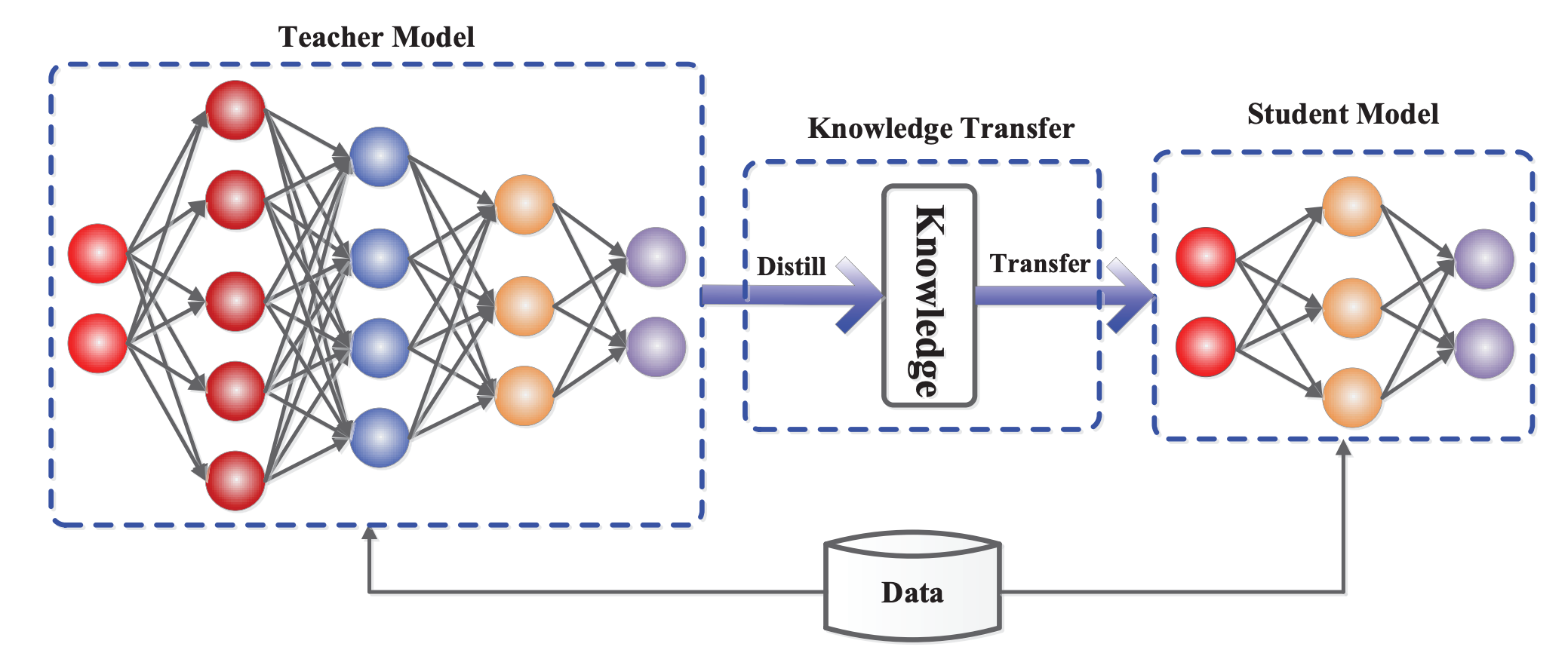
A knowledge distillation system consists of three principal components: the knowledge, the distillation algorithm, and the teacher-student architecture.
Knowledge distillation aims at creating a smaller student model from a large, complex teacher model. The initution is that the student model will have similar performance to the larger model, while still keeping model parameters and size significantly smaller compared to the original (teacher) model.
knowledge distillation typically involves the following:
- First, a large and accurate model is trained on the target task using a large dataset and significant computational resources. This trained model with high performance serves as the teacher.
- Next, a smaller and more efficient model architecture is defined, known as the student. This model is designed to be more lightweight and suitable for deploying on resource-constrained devices or environments.
- Then, the knowledge from the teacher model is then transferred to the student model through a training process. This is typically done by minimizing the difference between the outputs (logits or softmax probabilities) of the teacher and student models on the same input data. The student model is trained to mimic the behavior of the teacher model, effectively learning to approximate the teacher’s decision boundaries.
- Finally, after the initial knowledge transfer, the student model can be further fine-tuned on the target task using the original training data. This helps the student model to adapt to the specific task and recover any performance loss that may have occurred during the knowledge distillation process.

The generic teacher-student framework for knowledge distillation. Image Source
To learn more about various types of knowledge distillation, refer to this blog post.
Model Quantization Link to heading
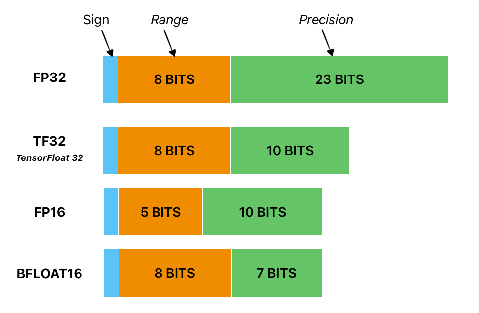
The size of a model is determined by the number of its parameters, and their precision, typically one of float32, float16 or bfloat16.
Model quantization is a process that involves converting the numerical precision of the parameters in a neural network from a higher precision format, such as 32-bit floating-point, to a lower precision format, like 8-bit integers.

Quantization reduces the bit-widths of computations and tensor storage, allowing for a more compact model representation and the use of high-performance vectorized operations on various hardware platforms.
A quantized model performs operations using integers rather than floating-point values, which can significantly improve inference speed and reduce computational costs.
Quantization Techniques Link to heading
Quantization can be applied during both training or post-training phases. Post-training quantization (PTQ) involves quantizing a fully trained model, which is straight forward but can lead to accuracy loss.
Quantization techniques applied during the training phase is often referred to as Quantization-Aware Training (QAT). Accuracy losses with QAT are much smaller compared to PTQ techniques.
While the process of quantization can be straight forward the choice of quantization technique depends on how much accuracy loss are you willing to accept for a given quantized model.
We could quantized a model to the lowest supported precision which could significantly reduce the model size and therefore computational requirements for hosting the model. However, is the accuracy drop reasonable and acceptable to host in the real-world will be the deciding factor.
There are many quantization techniques (PTQ) out there, each technique aims at reducing the accuracy loss by employing various techniques. Also, PTQ techniques are the most common and the easiest way to achieve inference performance for Large Language Models (LLMs).
Note: Quantization techniques outlined in this post are by no means exhaustive. Quantization remains an active research area in machine learning
In the next post, we’ll discuss a few popular PTQ techniques employed in the field for improving inference performance.